Detection/Inference
This guide covers how to use the trained model for detection and inference on spectrogram images.
Repository: GitHub
Pre-trained Models: Google Drive
Detection Overview
Detection involves:
- Loading a trained model
- Processing input images
- Running inference
- Post-processing detections
- Saving or visualizing results
Basic Detection
Simple Detection Command
python detect.py \
    --weights runs/train/exp28/weights/best.pt \
    --source path/to/images \
    --imgsz 512
This will:
- Load the trained model
- Process images from the source directory
- Save detection results to
runs/detect/exp/
Detection Parameters
Required Parameters
--weights: Path to model weights file
--weights runs/train/exp28/weights/best.pt
--source: Input source (file, directory, URL, or webcam)
--source path/to/images          # Directory
--source path/to/image.png       # Single image
--source 0                       # Webcam
--source https://example.com/img.jpg  # URL
Image Processing Parameters
--imgsz: Inference image size (must match training size)
--imgsz 512 # 512×512 pixels
--conf-thres: Confidence threshold (0.0-1.0)
--conf-thres 0.25  # Default: 0.25
--conf-thres 0.5   # Higher confidence
--conf-thres 0.932 # Very high confidence (100% precision)
--iou-thres: Non-Maximum Suppression IoU threshold
--iou-thres 0.45 # Default: 0.45
--max-det: Maximum detections per image
--max-det 1000 # Default: 1000
Output Parameters
--save-img: Save detection result images
--save-img true
--save-txt: Save detection labels in YOLO format
--save-txt
--save-conf: Include confidence scores in saved labels
--save-txt --save-conf
--project: Project directory for saving results
--project runs/detect
--name: Experiment name
--name exp
Visualization Parameters
--line-thickness: Bounding box line thickness
--line-thickness 3 # Default: 3
--hide-labels: Hide class labels on images
--hide-labels
--hide-conf: Hide confidence scores on images
--hide-conf
Advanced Parameters
--classes: Filter detections by class IDs
--classes 0 2 3 # Only detect classes 0, 2, 3
--agnostic-nms: Class-agnostic Non-Maximum Suppression
--agnostic-nms
--augment: Augmented inference (TTA - Test Time Augmentation)
--augment
--half: Use FP16 half-precision inference
--half # Faster, less accurate
--device: Device selection
--device 0        # GPU 0
--device 0,1,2,3  # Multiple GPUs
--device cpu      # CPU
Detection Examples
Example 1: Basic Detection
python detect.py \
    --weights runs/train/exp28/weights/best.pt \
    --source data/test_images \
    --imgsz 512 \
    --conf-thres 0.25 \
    --save-img true
Example 2: High Confidence Detection
For high-precision detection (100% precision at 0.932 confidence):
python detect.py \
    --weights runs/train/exp28/weights/best.pt \
    --source data/test_images \
    --imgsz 512 \
    --conf-thres 0.932 \
    --save-img true
Example 3: Save Labels
Save detection results in YOLO format:
python detect.py \
    --weights runs/train/exp28/weights/best.pt \
    --source data/test_images \
    --imgsz 512 \
    --save-txt \
    --save-conf
Example 4: Filter by Class
Detect only specific signal types:
python detect.py \
    --weights runs/train/exp28/weights/best.pt \
    --source data/test_images \
    --imgsz 512 \
    --classes 9 10  # LFM (9) and FMCW (10)
Example 5: Augmented Inference
Use Test Time Augmentation for better accuracy:
python detect.py \
    --weights runs/train/exp28/weights/best.pt \
    --source data/test_images \
    --imgsz 512 \
    --augment
Detection Output
Output Structure
Detection results are saved to:
runs/detect/exp/
├── image1.png      # Detection result image
├── image2.png
├── ...
└── labels/         # If --save-txt
    ├── image1.txt  # Detection labels
    ├── image2.txt
    └── ...
Detection Format
Image Output:
- Original image with bounding boxes
- Class labels and confidence scores
- Color-coded by class
Label Output (YOLO format):
class_id x_center y_center width height confidence
Example:
0 0.5 0.5 0.3 0.4 0.95
9 0.2 0.3 0.15 0.2 0.87
Detection Results
Sample Detection Images
The model successfully detects various signal types:
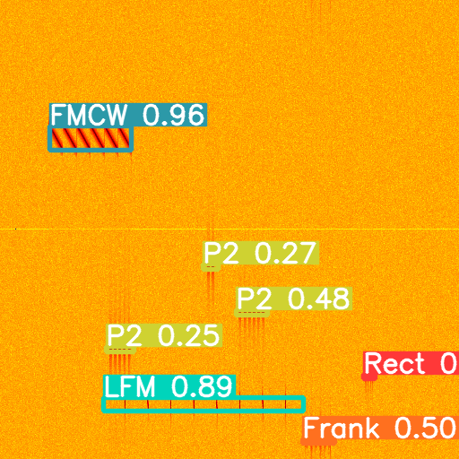
Multiple signal types detected in a single spectrogram
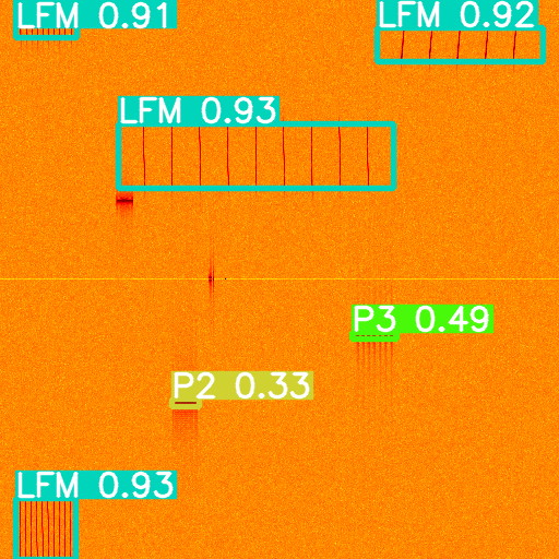
Various signal types with different confidence levels
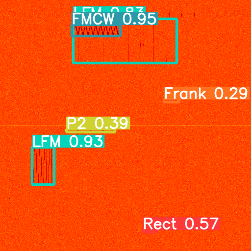
High-confidence detections in complex spectrogram environments
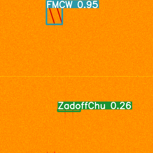
Detection in dense signal environments with multiple overlapping signals
Performance Considerations
Inference Speed
- Image Size: Larger images = slower inference
- Batch Size: Process multiple images for better GPU utilization
- Device: GPU is much faster than CPU
- Half Precision: Use
--halffor faster inference (slight accuracy loss)
Memory Usage
- Image Size: Larger images require more GPU memory
- Batch Processing: Process images one at a time for low memory usage
- Model Size: Larger models require more memory
Accuracy vs Speed Trade-off
- High Confidence (0.9+): Slower (fewer detections), very accurate
- Medium Confidence (0.25-0.5): Balanced speed and accuracy
- Low Confidence (<0.25): Faster (more detections), may include false positives
Confidence Threshold Selection
Based on the Precision-Confidence curve:
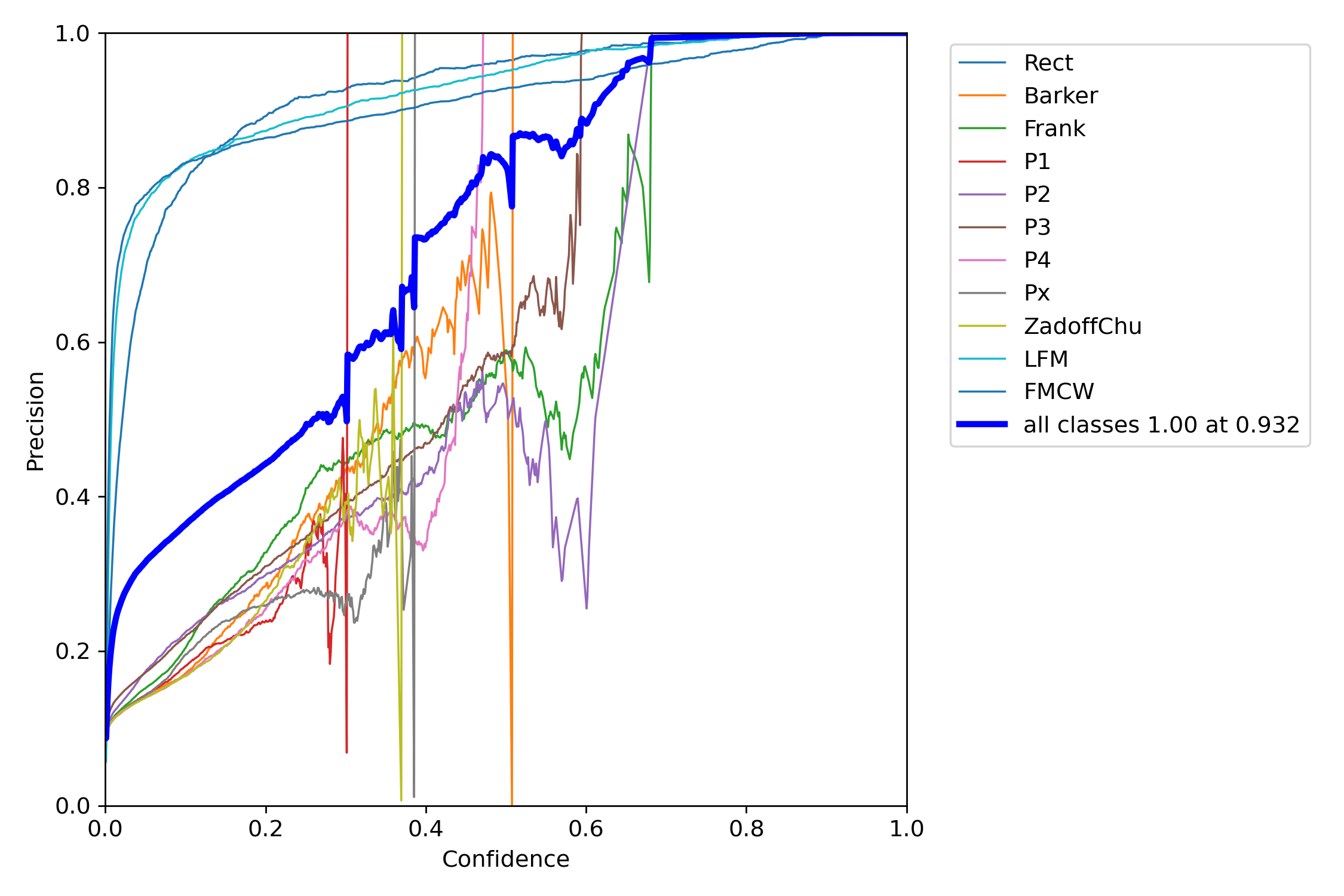
- 0.932: 100% precision (very reliable, fewer detections)
- 0.6-0.8: High precision (>80%), good balance
- 0.25-0.5: Moderate precision, more detections
- <0.25: Lower precision, many detections (may include false positives)
Best Practices
For High Precision
Use high confidence threshold:
--conf-thres 0.932 # 100% precision
For High Recall
Use lower confidence threshold:
--conf-thres 0.25 # More detections
For Balanced Performance
Use medium confidence threshold:
--conf-thres 0.5 # Good balance
Batch Processing
Process entire directories:
--source path/to/image/directory
Save Results
Always save results for analysis:
--save-img true --save-txt --save-conf
Troubleshooting
No Detections
- Lower confidence threshold
- Check image preprocessing
- Verify model was trained on similar data
- Check image size matches training size
Too Many False Positives
- Increase confidence threshold
- Adjust IoU threshold
- Use class filtering
- Check model training quality
Slow Inference
- Use GPU instead of CPU
- Reduce image size
- Use half precision (
--half) - Process in batches
Related Documentation
- Training: Training models for detection
- Configuration: Detection configuration options
- Architecture: Understanding the model architecture
- RadDet Use Case: Detection examples with RadDet dataset
- Model Conversion: Converting models for deployment
- Quantization: Optimizing models for faster inference