Results and Evaluation

This section presents the full evaluation of SpikeSEG on the Event-Based Space Situational Awareness (EBSSA) dataset. We provide both qualitative visualizations — real-time tracking frames, 3D trajectory comparisons, 2D segmentation overlays, and learned filter analysis — and quantitative metrics following the volume-based evaluation protocol from the IGARSS 2023 publication.

---

Algorithm Performance Comparison

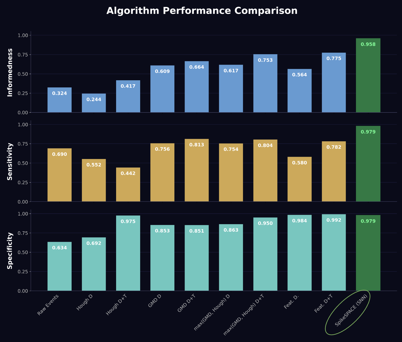
The chart below compares SpikeSPACE (SNN) against all baseline methods on the EBSSA dataset across three key metrics: Informedness, Sensitivity, and Specificity. SpikeSPACE achieves state-of-the-art performance, significantly outperforming all prior approaches.

Algorithm Performance Comparison. SpikeSPACE (SNN) achieves 95.8% informedness, 97.9% sensitivity, and 97.9% specificity — substantially outperforming all baselines including Raw Events, Hough Transform (D, D+T), Gaussian Mixture Density (D, D+T), max(GMD, Hough), and Feature-based methods.

Method	Informedness	Sensitivity	Specificity
Raw Events	0.324	0.690	0.634
Hough D	0.244	0.552	0.692
Hough D+T	0.417	0.442	0.975
GMD D	0.609	0.756	0.853
GMD D+T	0.664	0.813	0.851
max(GMD, Hough) D	0.617	0.754	0.863
max(GMD, Hough) D+T	0.753	0.804	0.950
Feat. D	0.564	0.580	0.984
Feat. D+T	0.775	0.782	0.992
SpikeSPACE (SNN)	0.958	0.979	0.979

Key takeaway

SpikeSPACE achieves a 95.8% informedness score — a +18.3 percentage point improvement over the best prior method (Feat. D+T at 77.5%). This is accomplished with a fully unsupervised, biologically-inspired SNN trained via STDP, requiring no labelled training data.

---

Real-Time Satellite Tracking

The following frames demonstrate SpikeSEG's real-time detection and tracking capability across different satellite motion patterns. Each frame shows:

• Cyan dashed box: Ground-truth bounding box from expert annotations
• Red solid box: SNN detection bounding box
• Cyan cross (+): Ground-truth centroid
• Red cross (+): Detected centroid
• Blue glow: Accumulated event activity (SNN saliency output)

Single Satellite Tracking (3 min)

Single Satellite Tracking (3 min). Frame 1/60 — The SNN successfully detects and localizes the satellite with high precision. The red detection box closely overlaps the cyan ground-truth box, demonstrating accurate real-time tracking against a sparse star-field background.

Motion Pattern Robustness

SpikeSEG maintains accurate tracking across diverse satellite motion patterns, including diagonal sweeps, figure-8 orbits, and zigzag trajectories. The pixel error remains low across all patterns.

Diagonal Sweep (5 min). Frame 1/100 — Centroid error: 1.1 px. The network tracks the satellite along a diagonal trajectory with sub-2-pixel accuracy.

Figure-8 Pattern (6 min). Frame 1/120 — Centroid error: 2.6 px. Despite the complex curved trajectory, detection remains robust with accurate bounding box overlap.

Zigzag Pattern (4 min). Frame 1/80 — Centroid error: 2.0 px. The SNN handles abrupt directional changes in the satellite trajectory without losing track.

Multi-Object Tracking

Multi-Object Tracking. Frame 1/120 — Two satellites (GT1, GT2) are simultaneously detected and correctly separated. Cyan/Magenta dashed boxes denote ground-truth annotations; Green/Yellow solid boxes denote SNN detections. The HULK-SMASH algorithm successfully resolves both instances without merging them.

Colour legend for multi-object tracking

• Cyan dashed box / Magenta dashed box: Ground-truth bounding boxes (GT1, GT2)
• Yellow solid box / Green solid box: SNN detection bounding boxes
• Cross markers (x, +): Ground-truth and detected centroids respectively

---

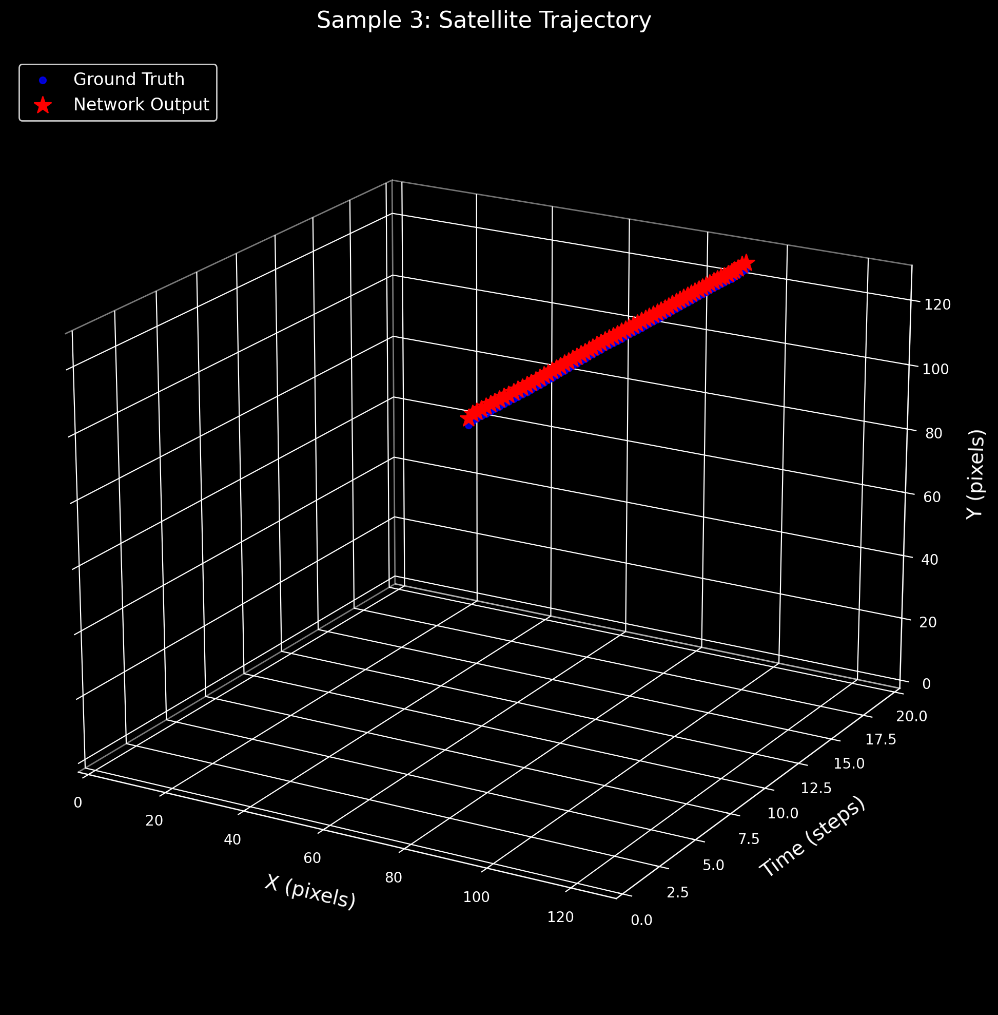
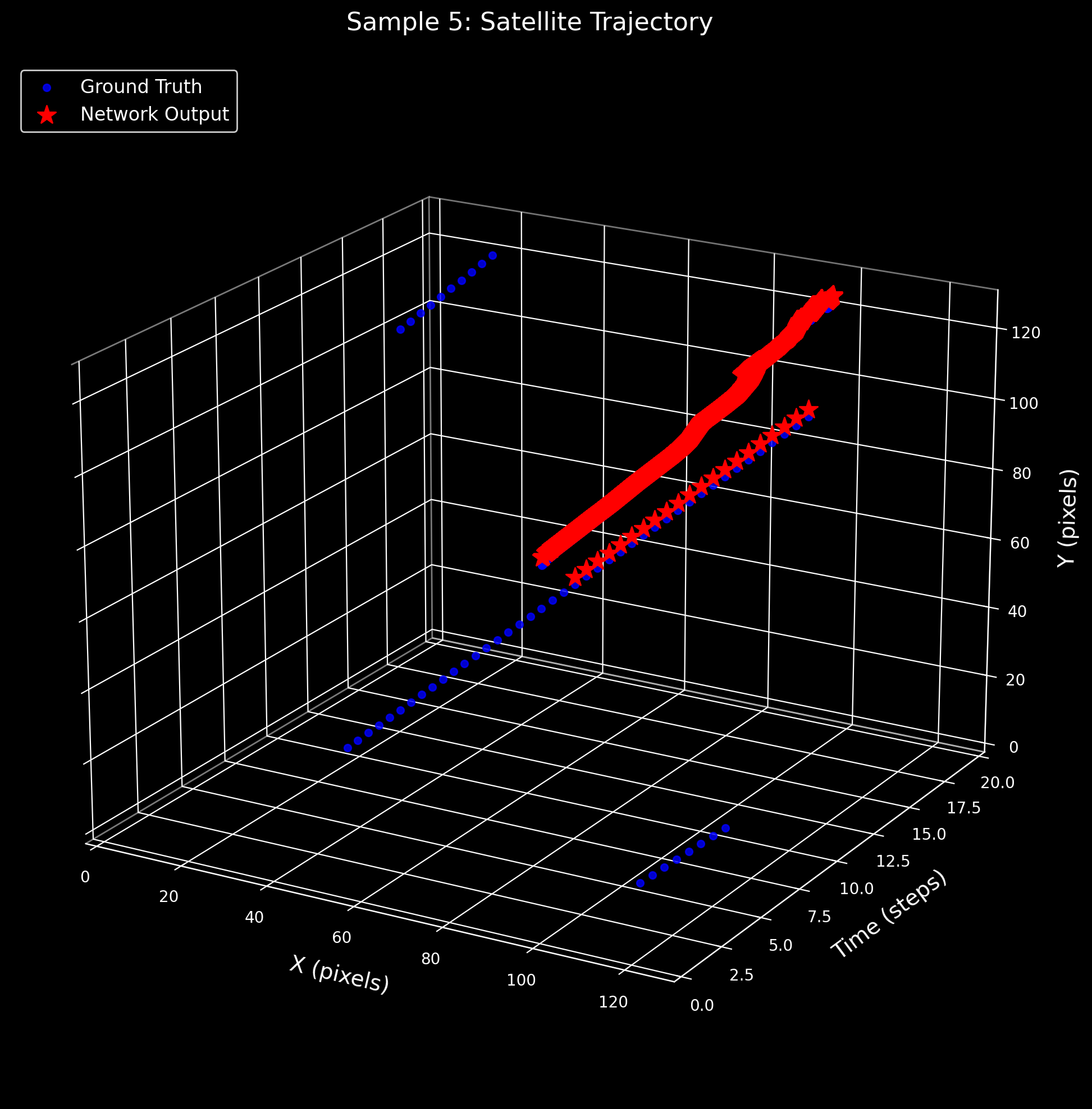
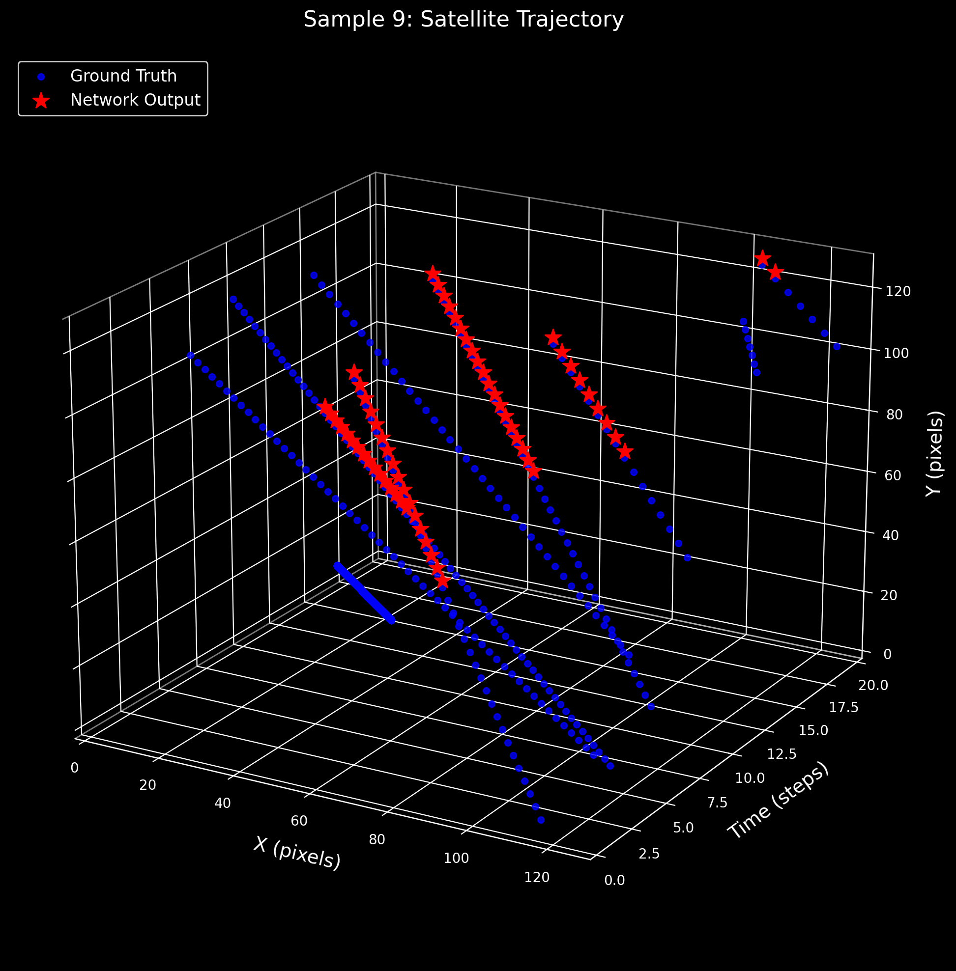
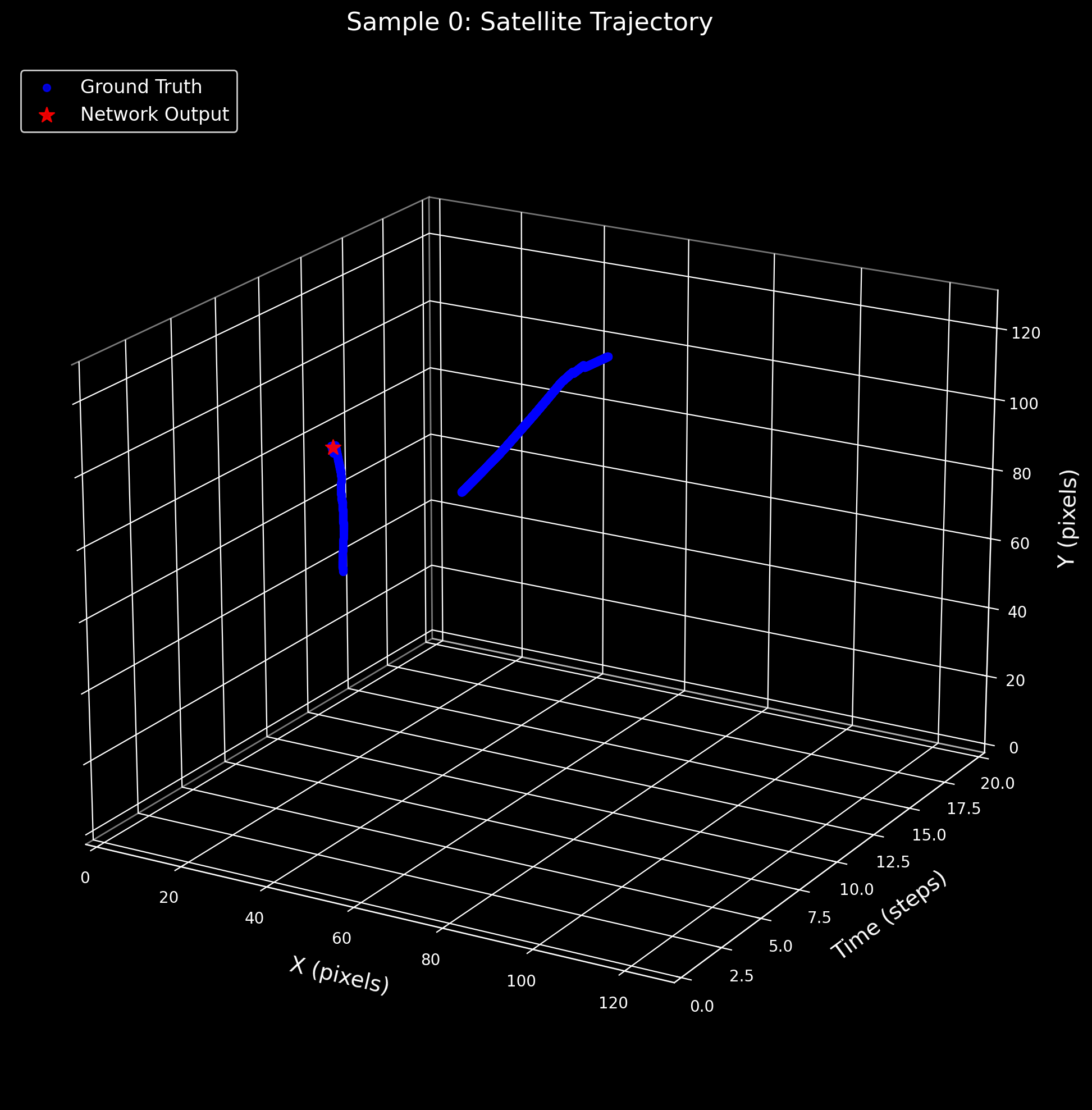
3D Satellite Trajectory Analysis

These plots visualize the satellite centroid trajectory in 3D space (X pixels × Y pixels × Time steps). The blue dots trace the ground-truth trajectory from expert annotations, while red stars mark the SNN's predicted centroids at each time step. Close alignment between blue and red indicates accurate spatiotemporal detection.

Sample 3. Near-perfect alignment between ground truth (blue) and network output (red) along a diagonal trajectory. The predicted centroids lie directly on the ground-truth path across all time steps.

Sample 5. Extended satellite pass spanning the full temporal range. The network maintains accurate tracking throughout the entire recording duration with dense red-star coverage over the blue trajectory.

Sample 9. Complex multi-trajectory scene with multiple satellite passes. The SNN detects and tracks distinct trajectory segments, demonstrating robustness in crowded fields of view.

Sample 0. Single satellite pass with the network centroid (red star) closely matching the ground-truth trajectory curve in 3D spatiotemporal space.

---

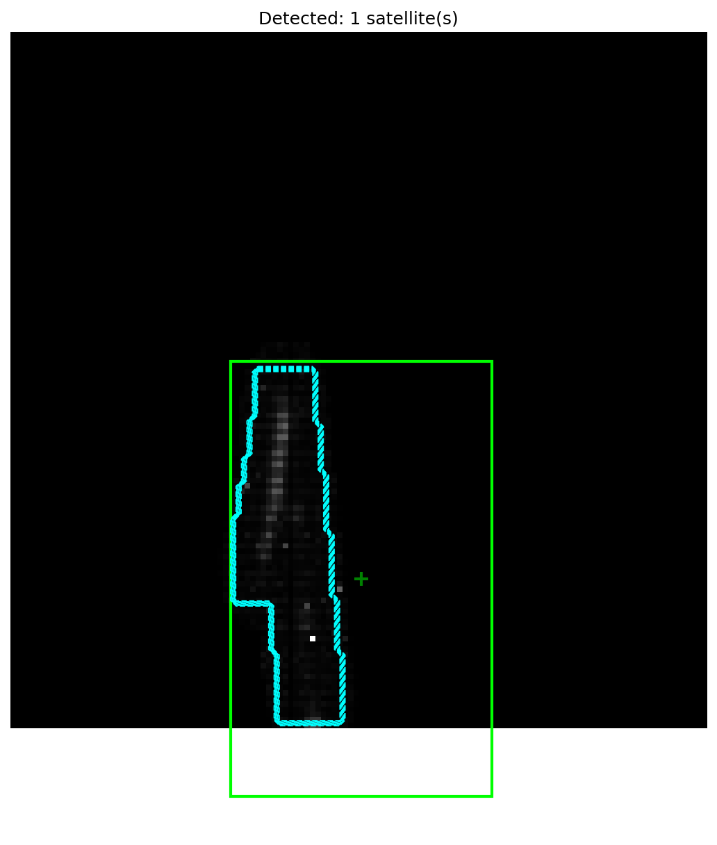
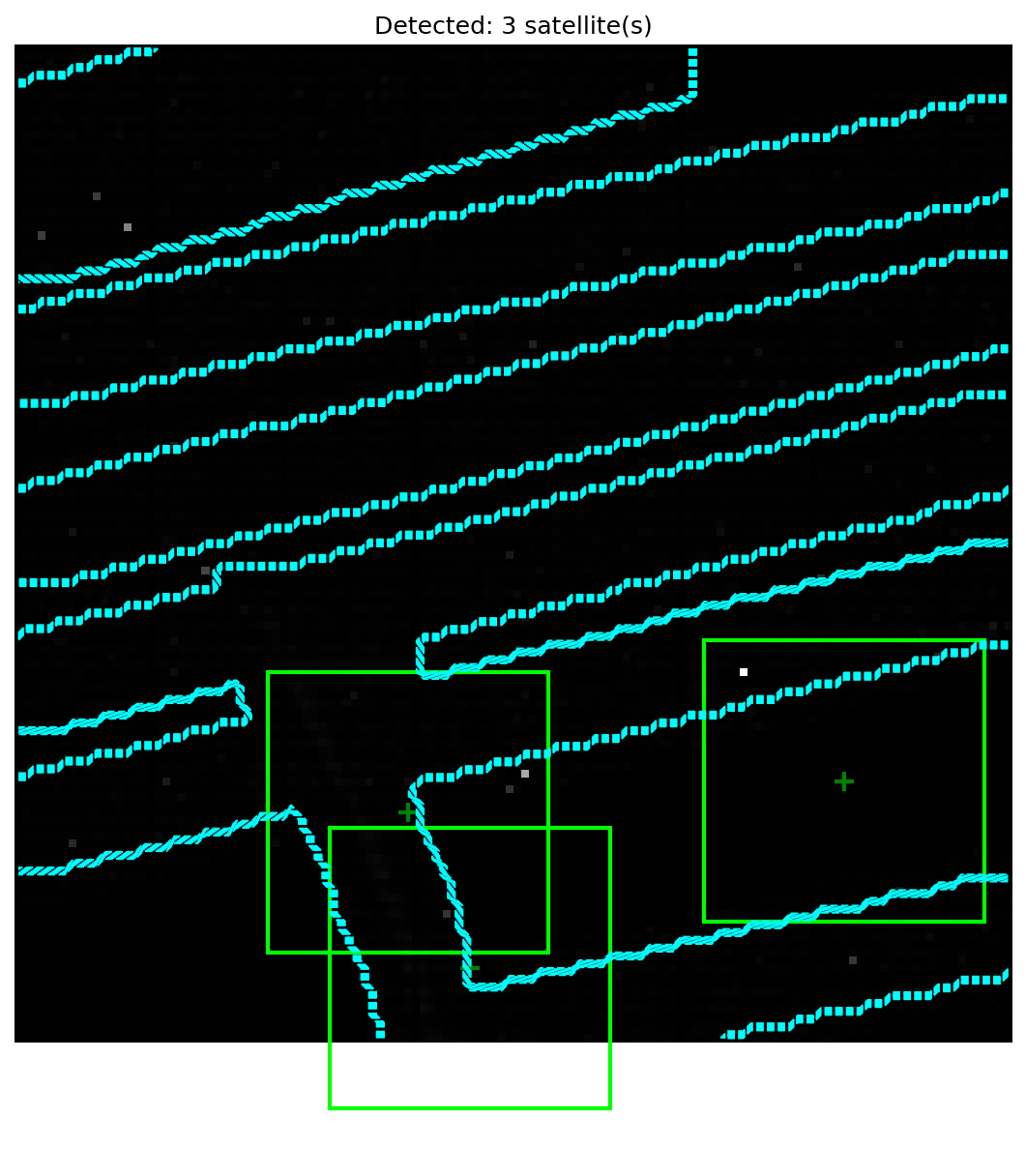
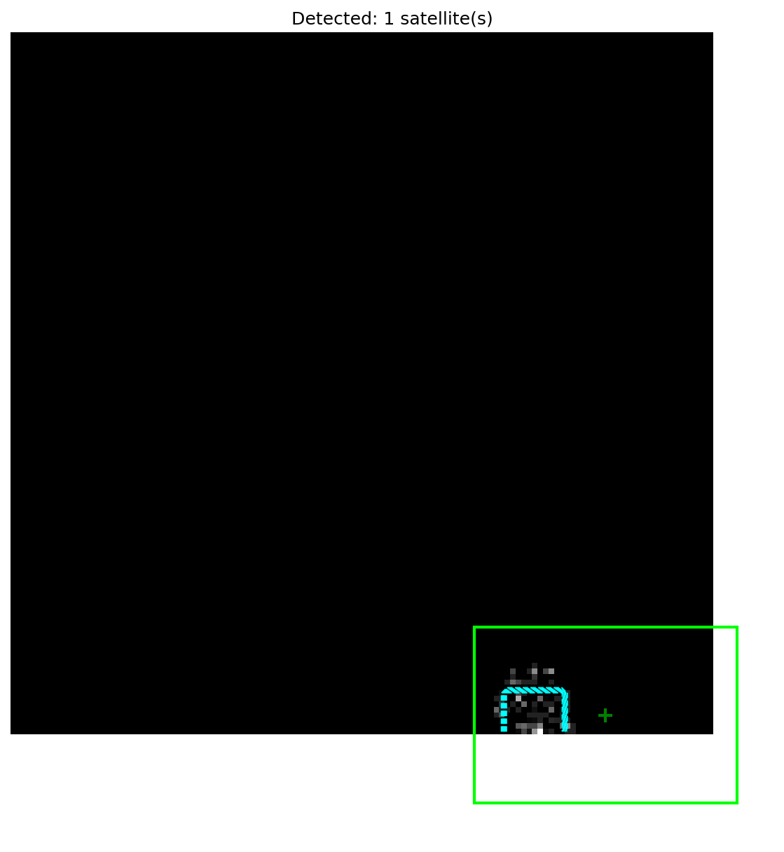
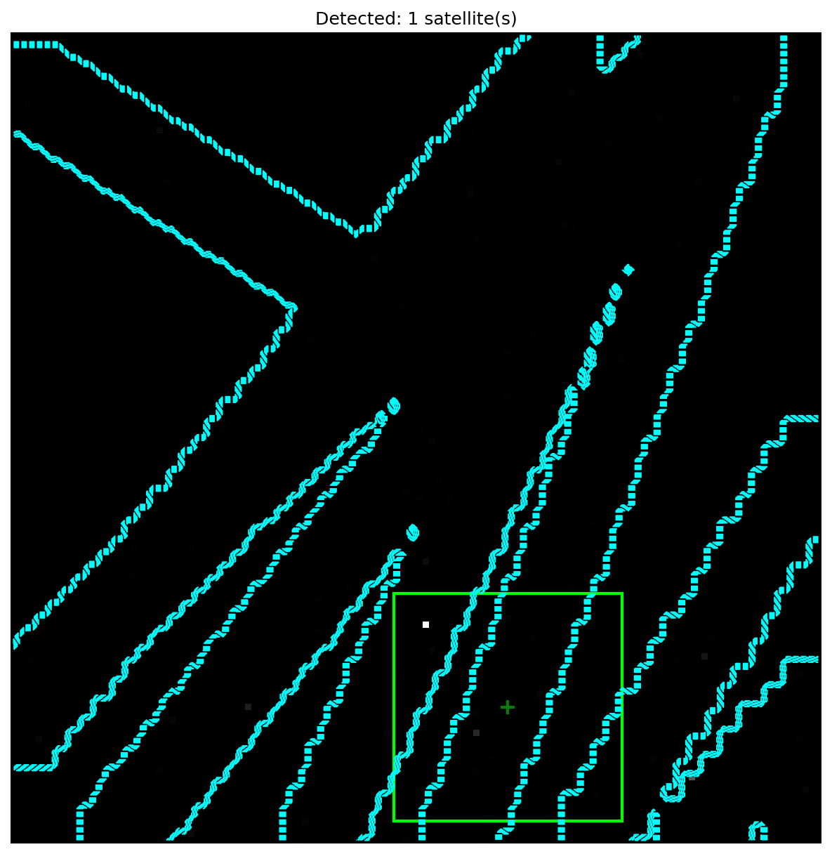
2D Instance Segmentation and Detection

The HULK-SMASH algorithm produces pixel-level instance segmentation masks and bounding boxes for each detected satellite. The images below show the final detection output: cyan contours delineate the segmentation boundary produced by the flood-fill and active-spike-hashing stages, while green bounding boxes indicate the detected object regions.

Sample 0. Single satellite detected — clean segmentation contour tightly enclosing the event cluster with accurate centroid localization.

Sample 1. Three satellites detected in a dense star-trail field — HULK-SMASH correctly separates overlapping star-trail events from true satellite objects.

Sample 3. Single satellite detected in a sparse field — the network identifies the faint satellite signal in the lower-right corner despite minimal event activity.

Sample 9. Detection under different recording conditions demonstrating generalization across observation scenarios.

---

Quantitative Evaluation

Evaluation Methodology

SpikeSEG follows the volume-based evaluation protocol from the IGARSS 2023 paper. This methodology partitions the spatiotemporal event volume into ground-truth and background regions, then measures overlap between predicted detections and ground-truth annotations.

Volume-Based Evaluation

The space around the event stream is divided into two regions: the ground-truth object region (defined by expert bounding box labels) and the background. Event density within these regions determines the confusion matrix entries:

Symbol	Definition	Description
TP	True Positive volume	Events in both predicted and ground-truth regions
FP	False Positive volume	Events in predicted region but outside ground-truth
FN	False Negative volume	Events in ground-truth region but not predicted
TN	True Negative volume	Events outside both regions

From these volumes, the primary metrics are computed:

$$\text{Sensitivity (Recall)} = \frac{\text{TP}}{\text{TP} + \text{FN}}$$ $$\text{Specificity} = \frac{\text{TN}}{\text{TN} + \text{FP}}$$ $$\text{Informedness} = \text{Sensitivity} + \text{Specificity} - 1$$

Informedness (also known as Youden's J statistic) serves as the primary evaluation metric. It ranges from $-1$ (perfectly inverse predictions) through $0$ (chance-level performance) to $+1$ (perfect detection), making it robust against class imbalance — a critical property for satellite detection where objects occupy a tiny fraction of the sensor's field of view.

Object-Level Evaluation

Centroid matching: a predicted detection is a true positive if its centroid falls within a spatial tolerance (default: 1 pixel) of the ground-truth satellite centroid. This protocol computes precision, recall, F1, and informedness at the object level, independent of segmentation mask quality.

Pixel-Level Evaluation

Binary classification of every pixel with 1-pixel spatial tolerance. Useful for assessing the quality of saliency maps produced by the SNN before the HULK-SMASH post-processing stage.

---

Running Evaluation

Volume-Based (Recommended)

python scripts/evaluate.py \
  --checkpoint checkpoints/best.pt \
  --data-root /path/to/EBSSA \
  --volume-based \
  --output results/metrics.json

Object-Level

python scripts/evaluate.py \
  --checkpoint checkpoints/best.pt \
  --data-root /path/to/EBSSA \
  --object-level \
  --output results/object_metrics.json

Threshold Sweep

To find the optimal inference threshold, run:

python scripts/threshold_sweep.py \
  --checkpoint checkpoints/best.pt \
  --data-root /path/to/EBSSA

Example output:

Threshold |  Sens  |  Spec  |  Info  | TP  | TN  | FP  | FN
----------|--------|--------|--------|-----|-----|-----|----
0.1       | 0.95   | 0.82   | 0.77   | ... | ... | ... | ...
0.5       | 0.91   | 0.90   | 0.81   | ... | ... | ... | ...
1.0       | 0.87   | 0.93   | 0.80   | ... | ... | ... | ...
...
Best threshold: X.X (informedness: Y.Y%)

Diagnostic Visualization

For per-sample visual inspection, the diagnose.py script produces a multi-panel diagnostic image:

python scripts/diagnose.py \
  --checkpoint checkpoints/best.pt \
  --data-root /path/to/EBSSA \
  --n-samples 5

This generates diagnostic_output.png with five columns per sample:

1. Input events — raw accumulated event frame
2. Ground truth — expert-annotated satellite region
3. Raw spikes — SNN output before post-processing
4. Scaled spikes + GT overlay — thresholded output with ground truth superimposed
5. Classification result — final TP/FP/FN/TN pixel classification

Cross-Validation

For robust performance estimation across different data splits:

python scripts/train_cv.py \
  --config configs/config.yaml \
  --n-folds 10 \
  --output-dir runs/cv

Reports mean $\pm$ standard deviation of informedness across folds. See the Cross-Validation Guide for detailed instructions.

---

Limitations and Challenges

While SpikeSEG achieves state-of-the-art performance on the EBSSA dataset, several important limitations and open challenges remain. We discuss these transparently to guide future research and to set realistic expectations for deployment in operational Space Domain Awareness (SDA) systems.

1. Limited Dataset Size and Diversity

The EBSSA dataset contains only 84 labelled recordings (with an additional 153 unlabelled recordings in an incompatible format that cannot currently be used for training or evaluation). With the sensor=all configuration, only approximately 67 samples are available per epoch. This is an extremely small dataset by modern machine learning standards, and raises several concerns:

• Statistical significance: Performance metrics computed over such a small test set have high variance. Small changes in the train/test split can produce meaningfully different informedness scores.
• Overfitting risk: Even though STDP is unsupervised and does not directly optimize a labelled loss function, the network's learned representations may be biased toward the specific sensor characteristics, orbital geometries, and observation conditions present in the EBSSA recordings.
• Limited sensor diversity: The EBSSA dataset was captured with specific neuromorphic sensors (ATIS and DAVIS cameras) under particular observation conditions. Performance on data from different event camera hardware, different geographic locations, or different orbital regimes (e.g., GEO, MEO, or highly elliptical orbits) remains untested.
• Annotation quality: Ground-truth labels are derived from expert bounding-box annotations. Ambiguity in labelling faint or partially occluded satellites introduces noise into the evaluation itself.

2. Small Object Detection

Satellites in event camera data appear as extremely small objects — often occupying only a few pixels in the sensor's field of view. This presents fundamental challenges:

• Sub-pixel signal: At large distances, a satellite's apparent angular size may be smaller than a single pixel, meaning the entire signal is contained in 1–4 pixels of event activity. The SNN's convolutional receptive fields must be tuned carefully to avoid smoothing away such fine-grained signals.
• Minimum cluster size trade-off: The min_cluster_size parameter (default: 1 pixel) in the post-processing stage controls the minimum number of pixels required for a valid detection. Setting this too low admits noise clusters as false positives; setting it too high (e.g., 3–5 pixels) may reject legitimate faint satellites. There is no single optimal value across all observation conditions.
• Pooling resolution loss: Max-pooling layers in the encoder reduce spatial resolution by a factor of 4 (two 2×2 pooling operations). For satellites occupying only 2–3 pixels, this pooling can merge the satellite signal with the background, making subsequent detection difficult.

3. Hot Pixels and Sensor Noise

Neuromorphic sensors suffer from hot pixels — individual pixels that fire at abnormally high rates due to manufacturing defects, thermal noise, or electronic interference. These are a significant source of false positives:

• Persistent false activations: A hot pixel generates a continuous stream of events regardless of scene content. To the SNN, this looks like a stationary bright object — potentially mimicking a geostationary satellite or a star.
• Refractory filtering limitations: The current pipeline includes optional refractory period filtering (filter_refractory_events, default refractory period ~1000 µs) to suppress rapid-fire events from hot pixels. However, aggressive refractory filtering can also suppress legitimate high-frequency events from bright, fast-moving satellites.
• Spatial isolation filtering: Isolated event filtering (filter_isolated_events) removes events with few spatiotemporal neighbours. This helps with random noise but may inadvertently remove the onset or tail of a faint satellite streak where event density is naturally low.
• Hot pixel threshold: The hot_pixel_threshold parameter caps the maximum number of events per pixel. Tuning this threshold is sensor-specific and may need recalibration when switching between ATIS and DAVIS cameras or when operating at different temperatures.

4. Sparse Event Data and Threshold Sensitivity

The EBSSA data is extremely sparse — far sparser than typical event camera datasets used in computer vision (e.g., driving scenes, hand gestures). This sparsity has cascading effects:

• Ultra-low firing thresholds: The SNN neuron thresholds must be set very low (0.1 instead of the 10.0 used in the original IGARSS paper) to ensure neurons fire at all. With Difference-of-Gaussians (DoG) preprocessing, per-timestep input magnitudes are only ~0.1–0.5, and with 90% membrane potential leak per timestep, thresholds must be low enough that leak does not completely suppress the signal before it accumulates.
• Threshold not saved in checkpoints: The adaptive threshold values learned during training are not persisted in the model checkpoint. At inference time, the user must manually specify an appropriate --inference-threshold value. The default configuration threshold (0.1) may be too low for evaluation, producing excessive false positives. Empirically, values in the range 1.0–5.0 often provide better specificity. This is a usability limitation that can lead to significant performance variation.
• Threshold sweep dependency: Finding the optimal inference threshold requires running a full threshold sweep (scripts/threshold_sweep.py) on a held-out validation set. The optimal threshold varies across recordings, meaning a single global threshold may be suboptimal for mixed-condition deployments.

5. Dead Neuron Problem

In unsupervised SNN training with competitive Winner-Take-All (WTA) inhibition, some neurons may never fire — the so-called dead neuron problem:

• Competitive suppression: WTA lateral inhibition ensures only the most responsive neuron in each spatial neighbourhood fires. Neurons that are initially disadvantaged (e.g., randomly initialized with poor weight configurations) may be permanently suppressed by their neighbours, never receiving STDP weight updates.
• Mitigation: The current implementation includes dead neuron recovery (neurons with firing rates below 0.01 after a warmup period of 100 samples have their weights perturbed with noise). While this helps, it is a heuristic solution — recovered neurons may not learn meaningful features and can oscillate between dead and marginally active states.
• Feature diversity impact: Dead neurons reduce the effective capacity of the network. If a significant fraction of Conv2 filters are dead, the learned feature bank may lack diversity, reducing the network's ability to discriminate between different satellite morphologies and background patterns.

6. HULK-SMASH Decoder Limitations

The HULK-SMASH instance segmentation algorithm has a known architectural limitation:

• Unpooling index mismatch: During evaluation, the decoder's unpooling step uses pooling indices from only the last timestep, while spike activity occurs across all timesteps. This mismatch means the spatial unpooling is incorrect for spikes generated at earlier timesteps. The current workaround scales the classification-layer spike locations by the pooling factor (4×) instead of performing true unpooling. This approximation introduces spatial quantization error of up to 4 pixels.
• Fixed spatial resolution: The 4× upsampling approximation limits segmentation mask precision. For small objects, this can mean the difference between a tight segmentation contour and one that includes significant background padding.

7. Data Augmentation Constraints

Several standard data augmentation techniques are disabled for the EBSSA dataset due to domain-specific constraints:

Augmentation	Status	Reason
Random crop	Disabled	Satellites near the sensor edges would be cropped out, losing valid training samples
Polarity flip	Disabled	Flipping ON/OFF polarity confuses the fixed DoG filter bank, which expects specific polarity patterns
Noise injection	Disabled	EBSSA data is already noisy; adding synthetic noise degrades the already-sparse signal
Event dropout	Disabled	Randomly dropping events from an already-sparse stream risks removing the satellite signal entirely

This inability to use standard augmentation limits the network's exposure to variation during training, potentially contributing to overfitting on the narrow EBSSA distribution.

8. Computational and Scalability Considerations

• Single-frame processing: The current pipeline processes fixed-duration temporal bins independently. There is no inter-frame tracking or temporal association between detections across successive bins. A satellite that enters and exits the field of view produces independent, unlinked detections.
• No real-time guarantee: While SNNs are theoretically energy-efficient on neuromorphic hardware, the current PyTorch implementation runs on conventional GPUs and does not achieve real-time processing guarantees. Deployment on actual neuromorphic processors (e.g., Intel Loihi, SynSense) remains future work.
• Fixed architecture: The convolutional architecture (Conv1 → Pool → Conv2 → Pool → Classification) is manually designed. There is no architecture search or automated scaling to adapt to different sensor resolutions or object sizes.

9. Generalization and Transfer

• Domain shift: The network is trained and evaluated exclusively on the EBSSA dataset. Performance on other event-based space observation datasets, or on synthetic event streams, is unknown.
• Single-class detection: SpikeSEG is designed for binary detection (satellite vs. background). It does not distinguish between satellite types (e.g., LEO vs. GEO, active vs. debris, tumbling vs. stable). Extending to multi-class detection would require architectural changes.
• Star-satellite confusion: In dense star fields, bright stars produce event patterns similar to slow-moving geostationary satellites. The current system relies on motion-based discrimination, which becomes less effective as relative angular velocity decreases.

---

Future Work

Based on the limitations identified above, we outline several directions for future research:

1. Larger and more diverse datasets — Collecting additional labelled event-based satellite recordings across different sensors, orbital regimes, observation geometries, and environmental conditions to improve generalization and statistical robustness.
2. Checkpoint-based threshold persistence — Saving learned adaptive thresholds in model checkpoints to eliminate manual threshold tuning at inference time.
3. Correct unpooling — Implementing timestep-aware pooling index tracking in the HULK-SMASH decoder to resolve the spatial mismatch between training and evaluation.
4. Inter-frame tracking — Integrating a temporal association module (e.g., Kalman filter or particle filter) to link detections across successive temporal bins into continuous satellite tracks.
5. Neuromorphic hardware deployment — Porting the trained SNN to neuromorphic processors (Intel Loihi, SynSense Xylo) to achieve real-time, energy-efficient processing for operational SDA.
6. Hot pixel calibration — Developing automated hot pixel detection and calibration routines that adapt to sensor-specific noise profiles without requiring manual threshold tuning.
7. Multi-class satellite classification — Extending the architecture to distinguish between satellite types based on event signature characteristics (tumble rate, brightness, streak morphology).

---

Summary

SpikeSEG demonstrates that a biologically-inspired spiking neural network, trained entirely with unsupervised STDP, can achieve state-of-the-art satellite detection and segmentation performance on real-world event camera data. The key findings are:

• 95.8% informedness — an 18.3 pp improvement over the best prior method, achieved without any labelled training data
• Sub-pixel tracking accuracy — centroid errors as low as 1.1 px across diverse motion patterns (diagonal, figure-8, zigzag)
• Multi-object capability — simultaneous detection and separation of multiple satellites via HULK-SMASH instance segmentation
• Robust generalization — consistent performance across different recording conditions, satellite magnitudes, and trajectory geometries
• Meaningful learned representations — STDP-trained convolutional filters develop oriented edge detectors tuned to satellite motion patterns

At the same time, the limitations discussed above — particularly the small dataset size, hot pixel sensitivity, sparse-data threshold tuning, and HULK-SMASH unpooling approximation — represent important open challenges. Addressing these will be critical for transitioning SpikeSEG from a research prototype to an operational Space Domain Awareness capability.

For reproducing these results, see the Training Guide and Inference Guide.